


👋 Claire here. I’ve been working with data for six years, and always in the context of a “Modern Data Stack” — the first data stack I used included Redshift, Fivetran and Looker! In contrast, many data modeling concepts were coined in an era when analysts used on-prem databases like Oracle and IBM.
As I got further into my career, I came across more terminology that didn’t make sense to me, and I was never sure whether it was because the concept was irrelevant for today’s tools, or whether it was a valuable concept that I just hadn’t wrapped my head around yet.
We’re going to do a series of posts on some of these concepts, especially for those that work with a modern data stack. Let us know if you find this useful, if there’s a concept you’d like explained, or just want to say hi! Oh and one last thing before we dive in — applications for our fall cohort are now open.
For the last few years, every time someone mentioned an OLAP cube, I nodded a little, quickly checked out the Wikipedia article, got to the section about the “Mathematical definition” and quickly tapped out — “better to just remain blissfully ignorant”, I decided.
When I went to source ideas for a glossary of these terms, I quickly learned that it’s not just me who struggled to understand this term.
So today, we’re going to actually find out what an OLAP cube is — I didn’t expect to go so deep on this topic, and yet here we are!
First, let’s break the name down:
- OLAP: online analytical processing — an OLAP system is one that is designed for queries (that you run online?) for the purpose of analytics. This is in contrast to an OLTP system (T for transactional), that is designed for transactional queries (insert this record, update that address etc. etc.). All we really need to know here is that “OLAP” signifies “pattern for analytics”
- Cube: yikes… we’ll come back to this cube concept in about 800 words’ time (promise!)
What actually are OLAP cubes?
Let’s say you get a request like this:
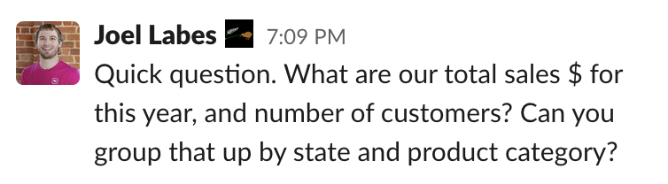
If you’re used to using a modern data stack, running a query like this isn’t so scary:
select
product_category,
state,
sum(sales) as total_sales_amount,
count(distinct customer_id) as number_of_customers
from sales
where date_trunc('year', sold_at) = 2021
group by 1, 2Code language: SQL (Structured Query Language) (sql)Rewind 10-20 years though, and this kind of query was really expensive¹ to run, especially when we have tens of thousands of sales each year. (There’s a lot more nuance to understand why modern data warehouses can handle this query, we might cover it in another post, but it has to do with row vs. columnar storage — this is a great primer)
The solution? Let’s pre-aggregate the data into a table! Sure you lose the ability to interrogate individual records, but it will be so much faster! (Sure we lose all the flexibility of querying our raw data, but back in 2001, we needed to do something like this)
| product_category | state | year | total_sales_amount | number_of_customers |
|---|---|---|---|---|
| brewing supplies | NY | 2021 | 612 | 27 |
| brewing supplies | VT | 2021 | 172 | 9 |
| coffee beans | NY | 2021 | 575 | 27 |
| coffee beans | VT | 2021 | 256 | 12 |
| merchandise | NY | 2021 | 415 | 16 |
| merchandise | VT | 2021 | 325 | 14 |
Perfect! Now our query is really quick to run:
select
  product_category,
  state,
  total_sales_amount,
  number_of_customers

from sales_cube
where year = 2021Code language: SQL (Structured Query Language) (sql)
That table we created? We can call that an OLAP cube.
In general, an OLAP cube is any pre-aggregated table that has multiple dimensions (things we group by) and measures (pre-aggregated numbers) on it. So really, it’s just a table. We’ll get to the “cube” name later on.
🚨 Common misunderstanding
At first I thought a “cube” was in the same class of things as a “table” or “view”, like a different storage mechanism in the database. This is not the case, it’s just a table, that’s used to power a particular kind of analysis.
Extending the pattern for more use cases
So, we send the results of our query to our stakeholder, and straight away get this request back…
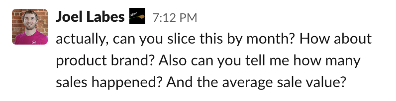
By this point, in 2021, we’re probably saying “oh crap, building this table was a mistake, I should have just given Joel the sales table and done the aggregates in the BI tool”. But, let’s keep going with our OLAP cube strategy.
Instead, the idea is to make the table have as many dimensions (things we group by) and measures (pre-aggregated numbers) as we might want to use in our reports:
| product_category | brand | state | month | year | total_sales_count | total_sales_amount | number_of_customers |
|---|---|---|---|---|---|---|---|
| coffee beans | brio | NY | January | 2021 | 3 | 57 | 2 |
| coffee beans | carrier | NY | January | 2021 | 2 | 22 | 2 |
| coffee beans | brio | VT | January | 2021 | 2 | 38 | 2 |
| coffee beans | carrier | VT | January | 2021 | 1 | 20 | 1 |
| … | … | … | … | … | … | … | … |
| coffee beans | brio | NY | February | 2021 | 4 | 52 | 3 |
| coffee beans | carrier | NY | February | 2021 | 1 | 10 | 1 |
| coffee beans | brio | VT | February | 2021 | 2 | 28 | 2 |
| coffee beans | carrier | VT | February | 2021 | 3 | 54 | 3 |
| … | … | … | … | … | … | … | … |
^ yup, also an OLAP cube, and one we’ll forever be updating as more requests come in!
But I know what you’re thinking, “I see no cubes, this is just a two dimensional table, but the Wikipedia article has lots of illustrations of cubes…”
So where does this “cube” term come from?
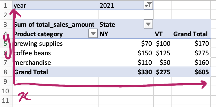
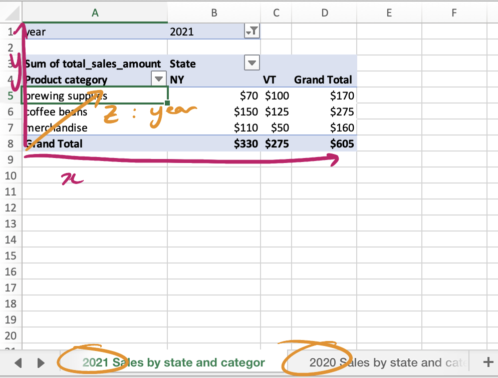
Back in 2001, our pre-aggregated table would be loaded into a world-class BI tool like Excel, and analyzed through Pivot Tables. Here, we have state along the x-axis, and product_category along the y-axis, with a filter for year = 2021. Each cell is populated with (the sum of) total_sales_amount.
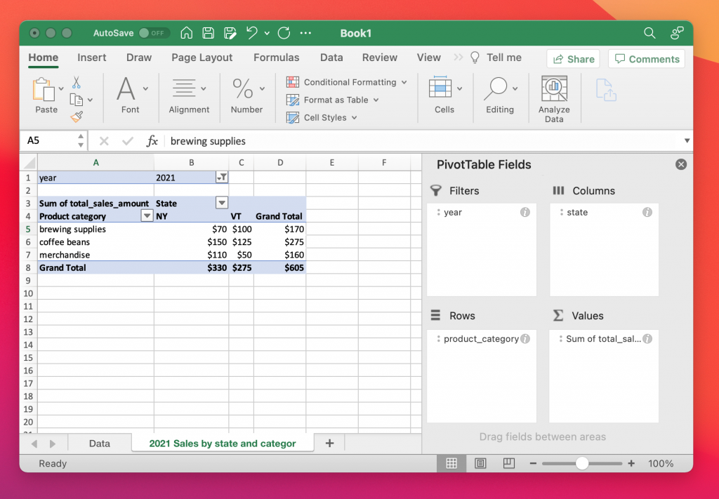
We can kind of see a “square” here (read: rectangle):
But when you’re using a pivot table to analyze data, you only get to play with two dimensions at once (product category x state). What if you instead wanted to analyze three dimensions at once? For example, how does our sales of coffee beans in NY in 2021 compare to the same category in 2020?
If you’re really great at Excel you might have an idea to stack multiple spreadsheet tabs on top of each other, one for each value of the third dimension (e.g. one tab for year = 2021, another for year = 2020, etc, etc). Thus creating a “cube” (read: rectangular prism) of pivot tables stacked on top of each other.
So the OLAP cube gets its name because it can be analyzed in this “cube-like” shape. Most of the time when someone is talking about “building a cube” they just mean building the underlying table that powers this kind of analysis.
Because many datasets will have more than three dimensions (things to group by), sometimes they will be called OLAP hypercubes. To that I say: (╯°□°)╯︵ ┻━┻
As far as I can tell, popular BI tools at the time had built-in features to view data this way, so you didn’t actually create one spreadsheet tab per value along the z-axis — I’ve just used Excel’s Pivot Tables here since most people are familiar with them, and it’s relatively easy to visualize the z-axis through different spreadsheet tabs.
And all those other terms?
Now that we kind of understand where the “cube” terminology comes from, we can introduce more ridiculous terminology:
- Slice: the dimensions that you analyze by along the z-axis. In our above example we “slice” by year.
- Dice: the dimensions on the x-axis or y-axis (yes, apparently these are distinct terms). Here we “dice” by product_category, and state
- Drill down: Expanding a dimension into a smaller sub-dimension, e.g. “slicing” by month instead of year, or “dicing” by county instead of state.
- Pivot the cube: rotating the cube, so perhaps “year” is on the x-axis, and “product category” is on the y-axis, meaning each tab shows a different “state”.
Handling non-additive aggregates
This section is probably only relevant if you choose / are forced to use this pattern (which hopefully you realize by now that I don’t recommend) — feel free to skip it if you want.
Let’s revisit our original table that we built: one record per state, per product category, per year.
| product_category | state | year | total_sales_amount | number_of_customers |
|---|---|---|---|---|
| brewing supplies | NY | 2021 | 612 | 27 |
| brewing supplies | VT | 2021 | 172 | 9 |
| coffee beans | NY | 2021 | 575 | 27 |
| coffee beans | VT | 2021 | 256 | 12 |
| merchandise | NY | 2021 | 415 | 16 |
| merchandise | VT | 2021 | 325 | 14 |
What happens when we only want to slice/dice/filter by a subset of those dimensions? For example, “2021 sales by state” (no mention of “product category”).
At first we try to use the table we just built, with a simple group by statement, to get our results.
select
state,
sum(total_sales_amount) as total_sales_amount,
???(number_of_customers) as number_of_customers
from sales_rollup
where year = 2021
group by 1
Code language: SQL (Structured Query Language) (sql)But straight away, we recognize a problem — the number of customers was built using a distinct count, and you can’t sum together two distinct counts².
🌠 The more you know: non additive aggregates
A distinct count is known as a “non-additive aggregate”. Other non-additive aggregates include averages and medians.
Should we create a new table excluding this product_category dimension? Like this?
| state | year | total_sales_amount | number_of_customers |
|---|---|---|---|
| NY | 2021 | 1602 | 54 |
| VT | 2021 | 753 | 28 |
Then we might also need a table excluding state, and then one that excludes year. What if… we could somehow … union these tables together to create one table that answers all the questions? 🤯
The most common solution is to pretty much do that — create a table as follows, using NULL values for the case when a dimension isn’t included in the final output:
| product_category | state | year | total_sales_amount | number_of_customers |
|---|---|---|---|---|
| brewing supplies | NY | 2021 | 612 | 27 |
| brewing supplies | VT | 2021 | 172 | 9 |
| coffee beans | NY | 2021 | 575 | 27 |
| coffee beans | VT | 2021 | 256 | 12 |
| merchandise | NY | 2021 | 415 | 16 |
| merchandise | VT | 2021 | 325 | 14 |
| brewing supplies | NULL | 2021 | 784 | 33 |
| coffee beans | NULL | 2021 | 831 | 35 |
| merchandise | NULL | 2021 | 740 | 27 |
| NULL | NY | 2021 | 1602 | 54 |
| NULL | VT | 2021 | 753 | 28 |
| NULL | NULL | 2021 | 2355 | 66 |
| … | … | … | … | … |
(The ... row represents that we need to repeat this NULL pattern for other years, excluded from this example for the sake of brevity).
Here’s how we would now write our original query (left), and the new request (right) with this structure — note the new where clauses: one for each dimension.
2021 sales by category x state:
select
  product_category,
  state,

  total_sales_amount

from sales_cube
-- the where clauses are new
where product_category is not null
  and state is not null
  and year = 2021Code language: SQL (Structured Query Language) (sql)
2021 sales by state:
select
  state,

  total_sales_amount


from sales_cube
-- use is null when a dimension is excluded
where product_category is null
  and state is not null
  and year = 2021
Code language: SQL (Structured Query Language) (sql)
💥 Boom! We just managed to make our one table return the correct number_of_customers, a non-additive aggregate, in both cases!
There’s even a special group by cube clause in some data warehouses to help generate this structure (Oracle and Snowflake³, but not Redshift nor BigQuery):
select
  product_category,
  state,
  date_trunc('year', sold_at) as date_year

  sum(sales) as total_sales_amount,
  count(distinct customer_id) as number_of_customers

from sales
group by cube(product_category, state, date_year)
Code language: SQL (Structured Query Language) (sql)
In reality though, modern BI tools aren’t built to consume this data structure, so while it’s clever, it’s not going to be that useful to your stakeholders who are using Looker or Mode for their queries.
The role of OLAP cubes in 2021
Today, the OLAP cube pattern is mostly irrelevant since data warehouses can handle aggregating your sales table on the fly. This patten does still offer two distinct advantages though
1. Queries on top of OLAP cubes are genuinely faster/cheaper than querying more granular data.
IMO, the cost saving usually isn’t worth it compared to the fact that you can’t actually drill down to the individual record. You’ll likely spend more money on human brain power creating these tables, than the money it costs to aggregate at query time.
Heads up: if you work at a company that has truly massive data, this advantage could become more relevant to you. If you take this approach, make sure you work with your stakeholders to pre-define what one record will represent (e.g. “one record per date per product category per state”), so that you don’t have to keep going back and adding dimensions later.
2. It’s much less common for two people to have different numbers for the same metric when using an OLAP cube.
This one is important.
In our example, our total_sales_amount is pre-computed, so we’re going to avoid two people defining sales as different numbers on a per-record level (does it include tax or not?), or using a different timezone to aggregate these numbers (are we using UTC, our head office time, or the local time of the store we sold things in?). OLAP cube proponents are generally holding on to this advantage as the reason to keep using this pattern.
While we can dream of having a sales table that is so well designed that our stakeholders just get the right answer when querying it themselves, if you’ve worked with data that’s got real-world complexity, you probably know that this dream is out of reach — someone is always going to find a way to mess it up.
Recently, there has been a lot of talk about a new solution to this problem — the “metrics layer” — a way to encode these metric definitions so aggregates at query time are always are calculated consistently. Benn Stancil summarizes it best in his recent blog post here, and tools like Transform are building a solution.
So, what is an OLAP cube?
A summary:
- An OLAP cube is a table that has multiple dimensions (columns you group by) and measures (pre-aggregated values). A better term might be “pre-aggregated table”.
- The name of this design pattern comes from:
- OLAP: pattern for analytics
- cube: these tables were often analyzed in Pivot Table-like structures, where the third dimension might be represented by stacking multiple Pivot Tables on top of each other, thus creating a “3D” representation of the data, or a “cube”
- The tradeoff of this design is that you can’t drill down all the way to the individual records and need to keep extending the pattern for every stakeholder’s request. Also, non-additive aggregates are challenging to deal with.
- To return the correct result for non-additive aggregates, sometimes OLAP cubes contain records with
NULLvalues to denote what the result should be when excluding a dimension from the results. Some warehouses havegroup by cubefunctions to create this structure. - The pattern is mostly irrelevant today since data warehouses in 2021 can handle running aggregates at query time
- However, pre-aggregated data did mean that there was only one way to calculate metrics, which is a missing layer of our current data stack. Tools in the “metrics layer” space seek to solve this.
Jargon as a gatekeeper
A few people were kind enough to read the draft of this post, and almost all of them had the same journey as me — they thought OLAP cubes were this intimidating concept, and the more they read, the less they understood, but it turns out that they aren’t that confusing in practice. This is a trend that I’ve seen a lot in data engineering / data modeling where jargon is used as a gatekeeper⁴.
This kind of gatekeeping is not doing the data community any favors — sure, “naming things is hard” and all that, but naming things in a way that confuses people — that’s irresponsible at best, and cruel at worst. We need to do better — I don’t know how we fix it, but I’m hoping articles like this is a step in the right direction.
¹Expensive here means “uses up a lot of your resources at once”. For example, when Slack slows down your MacBook Pro, you can say it’s an “expensive” program. On some data warehouses, expensive also means “costs more money”, since you pay per query.
²An unrelated example of summing distinct counts: In a class, 10 students have pet cats, and 15 students have pet dogs (and there’s no other pets, like goldfish or birds). How many students have pets? It would be incorrect to add these two numbers together to say “25 students have pets”, since some students might have both! Therefore, this is a non-additive aggregate. Instead we know that between 15 and 25 students have pets. In comparison, if we know that students in the classroom collectively owned 12 cats and 18 dogs, we can say they own 30 pets in total. This is an additive aggregate.
³Why does Snowflake support group by cube(), but not Redshift or BigQuery? Snowflake tend to go after Oracle customers — providing SQL parity with Oracle enables them to do this more easily. It’s a good strategy, but it means a lot of people migrate legacy SQL without considering whether it’s still the best approach with their new shiny Modern Data Stack.
⁴Hat tip to Benn Stancil for the phrase and Josh Devlin for the same conversation.